Our Sumif Excel Statements

By pressing ctrl+change+facility, this will certainly calculate as well as return value from several varieties, instead of simply private cells contributed to or multiplied by each other. Determining the sum, product, or quotient of individual cells is very easy-- just use the =SUM formula as well as go into the cells, worths, or variety of cells you intend to do that math on.

If you're wanting to locate overall sales earnings from a number of sold systems, as an example, the array formula in Excel is best for you. Right here's just how you 'd do it: To begin making use of the variety formula, type "=SUM," and in parentheses, go into the very first of two (or three, or 4) varieties of cells you want to increase together.

This stands for reproduction. Following this asterisk, enter your second variety of cells. You'll be multiplying this second variety of cells by the first. Your development in this formula should currently look like this: =AMOUNT(C 2: C 5 * D 2:D 5) Ready to press Get in? Not so quickly ... Due to the fact that this formula is so complicated, Excel gets a different keyboard command for selections.

This will identify your formula as a variety, covering your formula in brace characters as well as efficiently returning your item of both arrays incorporated. In revenue estimations, this can cut down on your time and effort significantly. See the last formula in the screenshot over. The MATTER formula in Excel is represented =COUNT(Beginning Cell: End Cell).

For instance, if there are eight cells with gone into worths in between A 1 and A 10, =MATTER(A 1: A 10) will return a worth of 8. The MATTER formula in Excel is especially useful for big spread sheets, where you wish to see the amount of cells have real entrances. Don't be deceived: This formula won't do any type of mathematics on the values of the cells themselves.

The Greatest Guide To Excel Formulas

Making use of the formula in strong over, you can quickly run a matter of energetic cells in your spread sheet. The outcome will look a something like this: To perform the typical formula in Excel, get in the worths, cells, or series of cells of which you're calculating the average in the layout, =AVERAGE(number 1, number 2, and so on) or =STANDARD(Start Worth: End Value).

Discovering the average of a variety of cells in Excel maintains you from needing to locate private sums and after that performing a different department formula on your total. Making use of =AVERAGE as your initial message access, you can allow Excel do all the work for you. For recommendation, the standard of a team of numbers amounts to the sum of those numbers, split by the variety of things because group.

This will return the sum of the values within a preferred series of cells that all meet one requirement. For example, =SUMIF(C 3: C 12,"> 70,000") would return the sum of worths in between cells C 3 and also C 12 from only the cells that are greater than 70,000. Allow's claim you desire to figure out the revenue you produced from a checklist of leads who are linked with certain area codes, or determine the amount of certain workers' salaries-- but only if they fall above a certain quantity.

With the SUMIF feature, it doesn't have to be-- you can easily build up the amount of cells that meet certain standards, like in the income instance above. The formula: =SUMIF(variety, criteria, [sum_range] Array: The array that is being checked using your requirements. Requirements: The standards that identify which cells in Criteria_range 1 will certainly be added with each other [Sum_range]: An optional variety of cells you're mosting likely to accumulate along with the initial Array entered.

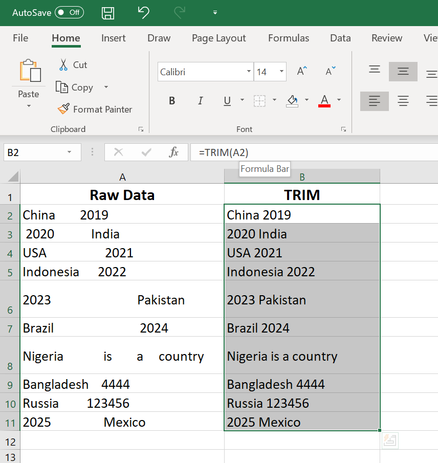
In the instance listed below, we intended to determine the sum of the salaries that were more than $70,000. The SUMIF feature built up the dollar amounts that went beyond that number in the cells C 3 via C 12, with the formula =SUMIF(C 3: C 12,"> 70,000"). The TRIM formula in Excel is denoted =TRIM(message).

3 Simple Techniques For Countif Excel

For instance, if A 2 includes the name" Steve Peterson" with undesirable spaces before the given name, =TRIM(A 2) would certainly return "Steve Peterson" with no rooms in a new cell. Email as well as file sharing are terrific tools in today's workplace. That is, till among your coworkers sends you a worksheet with some truly fashionable spacing.

As opposed to fastidiously eliminating and also including areas as required, you can clean up any kind of uneven spacing making use of the TRIM function, which is used to get rid of additional rooms from information (except for single rooms between words). The formula: =TRIM(text). Text: The text or cell from which you intend to get rid of rooms.

To do so, we got in =TRIM("A 2") into the Solution Bar, and replicated this for each and every name below it in a brand-new column beside the column with unwanted spaces. Below are a few other Excel formulas you could locate valuable as your data management requires grow. Allow's say you have a line of message within a cell that you wish to break down right into a few various sections.

Objective: Utilized to extract the very first X numbers or characters in a cell. The formula: =LEFT(message, number_of_characters) Text: The string that you desire to extract from. Number_of_characters: The number of characters that you want to remove beginning from the left-most character. In the example below, we entered =LEFT(A 2,4) right into cell B 2, and copied it into B 3: B 6.

Function: Used to extract personalities or numbers in the center based upon placement. The formula: =MID(message, start_position, number_of_characters) Text: The string that you wish to extract from. Start_position: The position in the string that you want to begin drawing out from. For instance, the very first setting in the string is 1.

The Greatest Guide To Excel Skills

In this instance, we went into =MID(A 2,5,2) right into cell B 2, and duplicated it into B 3: B 6. That enabled us to draw out both numbers beginning in the fifth placement of the code. Purpose: Used to extract the last X numbers or characters in a cell. The formula: =RIGHT(message, number_of_characters) Text: The string that you want to extract from.

excel formulas offset formula excel use same cell excel formulas how to use